Visualization
See the Gallery for more examples.
Output Formats
The show function is available in the axle._ package.
It can be applied to several types of Axle objects.
The package axle.awt._ contains functions for creating files from the images: png, jpeg, gif, bmp.
The package axle.web._ contains a svg function for creating svg files.
For example:
vis.show

vis.svg[IO]("filename.svg").unsafeRunSync()

vis.png[IO]("filename.png").unsafeRunSync()Animation
Plot, BarChart, BarChartGrouped, and ScatterPlot support animation.
The visualizing frame polls for updates at a rate of approximately 24 Hz (every 42 ms).
The play command requires the same first argument as show does.
Additionally, play requires a Observable[D] function that represents the stream of data updates.
The implicit argument is a monix.execution.Scheduler.
An axle.reactive.CurrentValueSubscriber based on the Observable[D] can be used to create the
dataFn read by the visualization.
See Bar Chart Animation for a full example of animation.
Plot
Two-dimensional plots
Example: Plot Random Waves Over Time
Imports
import org.joda.time.DateTime

import scala.collection.immutable.TreeMap
import scala.math.sin

import spire.random.Generator
import spire.random.Generator.rng

import cats.implicits._

import axle._
import axle.visualize._
import axle.joda.dateTimeOrder

import axle.visualize.Color._
Generate the time-series to plot
val now = new DateTime()

val colors = Vector(red, blue, green, yellow, orange)

def randomTimeSeries(i: Int, gen: Generator) = {
  val φ = gen.nextDouble()
  val A = gen.nextDouble()
  val ω = 0.1 / gen.nextDouble()
  ("series %d %1.2f %1.2f %1.2f".format(i, φ, A, ω),
    new TreeMap[DateTime, Double]() ++
      (0 to 100).map(t => (now.plusMinutes(2 * t) -> A * sin(ω * t + φ))).toMap)
}

val waves = (0 until 20).map(i => randomTimeSeries(i, rng)).toList
Imports for visualization
import cats.Show

import spire.algebra._

import axle.visualize.Plot
import axle.algebra.Plottable.doublePlottable
import axle.joda.dateTimeOrder
import axle.joda.dateTimePlottable
import axle.joda.dateTimeTics
import axle.joda.dateTimeDurationLengthSpace

implicit val fieldDouble: Field[Double] = spire.implicits.DoubleAlgebra
Define the visualization
val plot = Plot[String, DateTime, Double, TreeMap[DateTime, Double]](
  () => waves,
  connect = true,
  colorOf = s => colors(s.hash.abs % colors.length),
  title = Some("Random Waves"),
  xAxisLabel = Some("time (t)"),
  yAxis = Some(now),
  yAxisLabel = Some("A·sin(ω·t + φ)")).zeroXAxis
If instead we had supplied (Color, String) pairs, we would have needed something like preciding the Plot definition:
implicit val showCL: Show[(Color, String)] =
  new Show[(Color, String)] {
    def show(cl: (Color, String)): String = cl._2
  }
// showCL: Show[(Color, String)] = repl.MdocSession$App$$anon$1@399a70fc
Create the SVG
import axle.web._
import cats.effect._

plot.svg[IO]("docwork/images/random_waves.svg").unsafeRunSync()
Plot Animation
This example traces two "saw" functions vs time:
Imports
import org.joda.time.DateTime
import edu.uci.ics.jung.graph.DirectedSparseGraph
import collection.immutable.TreeMap

import cats.implicits._

import monix.reactive._

import spire.algebra.Field

import axle.jung._
import axle.quanta.Time
import axle.visualize._
import axle.reactive.intervalScan
Define stream of data updates refreshing every 500 milliseconds
val initialData = List(
  ("saw 1", new TreeMap[DateTime, Double]()),
  ("saw 2", new TreeMap[DateTime, Double]())
)
// initialData: List[(String, TreeMap[DateTime, Double])] = List(
//   ("saw 1", TreeMap()),
//   ("saw 2", TreeMap())
// )

val saw1 = (t: Long) => (t % 10000) / 10000d
// saw1: Long => Double = <function1>
val saw2 = (t: Long) => (t % 100000) / 50000d
// saw2: Long => Double = <function1>

val fs = List(saw1, saw2)
// fs: List[Long => Double] = List(<function1>, <function1>)

val refreshFn = (previous: List[(String, TreeMap[DateTime, Double])]) => {
  val now = new DateTime()
  previous.zip(fs).map({ case (old, f) => (old._1, old._2 ++ Vector(now -> f(now.getMillis))) })
}
// refreshFn: List[(String, TreeMap[DateTime, Double])] => List[(String, TreeMap[DateTime, Double])] = <function1>

implicit val timeConverter = {
  import axle.algebra.modules.doubleRationalModule
  Time.converterGraphK2[Double, DirectedSparseGraph]
}
// timeConverter: quanta.UnitConverterGraph[Time, Double, DirectedSparseGraph[quanta.UnitOfMeasurement[Time], Double => Double]] with quanta.TimeConverter[Double] = axle.quanta.Time$$anon$1@55b22c62
import timeConverter.millisecond

val dataUpdates: Observable[Seq[(String, TreeMap[DateTime, Double])]] =
  intervalScan(initialData, refreshFn, 500d *: millisecond)
// dataUpdates: Observable[Seq[(String, TreeMap[DateTime, Double])]] = monix.reactive.internal.operators.ScanObservable@239d3f0b
Create CurrentValueSubscriber, which will be used by the Plot to get the latest values
import monix.execution.Scheduler.Implicits.global
import axle.reactive.CurrentValueSubscriber

val cvSub = new CurrentValueSubscriber[Seq[(String, TreeMap[DateTime, Double])]]()
val cvCancellable = dataUpdates.subscribe(cvSub)

val plot = Plot[DateTime, Double, TreeMap[DateTime, Double]](
  () => cvSub.currentValue.getOrElse(initialData),
  connect = true,
  colorOf = (label: String) => Color.black,
  title = Some("Saws"),
  xAxis = Some(0d),
  xAxisLabel = Some("time (t)"),
  yAxisLabel = Some("y")
)
Animate
import axle.awt._

val (frame, paintCancellable) = play(plot, dataUpdates)
Tear down resources
paintCancellable.cancel()
cvCancellable.cancel()
frame.dispose()ScatterPlot
import axle.visualize._

val data = Map(
  (1, 1) -> 0,
  (2, 2) -> 0,
  (3, 3) -> 0,
  (2, 1) -> 1,
  (3, 2) -> 1,
  (0, 1) -> 2,
  (0, 2) -> 2,
  (1, 3) -> 2)
Define the ScatterPlot
import axle.visualize.Color._
import cats.implicits._
val plot = ScatterPlot[String, Int, Int, Map[(Int, Int), Int]](
() => data,
colorOf = (x: Int, y: Int) => data((x, y)) match {
case 0 => red
case 1 => blue
case 2 => green
},
labelOf = (x: Int, y: Int) => data.get((x, y)).map(s => (s.toString, false)))Create the SVG
import axle.web._
import cats.effect._

plot.svg[IO]("docwork/images/scatter.svg").unsafeRunSync()
BarChart
Two-dimensional bar charts.
Example: Fruit Sales BarChart
The dataset:
val sales = Map(
  "apple" -> 83.8,
  "banana" -> 77.9,
  "coconut" -> 10.1
)
Define a bar chart visualization
import spire.algebra.Field
import cats.implicits._
import axle.visualize.BarChart
import axle.visualize.Color.lightGray
implicit val fieldDouble: Field[Double] = spire.implicits.DoubleAlgebra
val chart = BarChart[String, Double, Map[String, Double], String](
() => sales,
title = Some("fruit sales"),
hoverOf = (c: String) => Some(c),
linkOf = (c: String) => Some((new java.net.URL(s"http://wikipedia.org/wiki/$c"), lightGray))
)Create the SVG
import axle.web._
import cats.effect._

chart.svg[IO]("docwork/images/fruitsales.svg").unsafeRunSync()
BarChart Animation
This example keeps the "bar" value steady at 1.0 while assigning a new random Double (between 0 and 1) to "foo" every second.
Imports
import scala.util.Random.nextDouble
import axle.jung._
import axle.quanta.Time
import edu.uci.ics.jung.graph.DirectedSparseGraph
import monix.reactive._
import axle.reactive.intervalScan
Define stream of data updates
val groups = Vector("foo", "bar")
val initial = Map("foo" -> 1d, "bar" -> 1d)

val tick = (previous: Map[String, Double]) => previous + ("foo" -> nextDouble())

implicit val timeConverter = {
  import axle.algebra.modules.doubleRationalModule
  Time.converterGraphK2[Double, DirectedSparseGraph]
}
import timeConverter.second

val dataUpdates: Observable[Map[String, Double]] = intervalScan(initial, tick, 1d *: second)
Create CurrentValueSubscriber, which will be used by the BarChart to get the latest value
import axle.reactive.CurrentValueSubscriber
import monix.execution.Scheduler.Implicits.global

val cvSub = new CurrentValueSubscriber[Map[String, Double]]()
val cvCancellable = dataUpdates.subscribe(cvSub)

import axle.visualize.BarChart

val chart = BarChart[String, Double, Map[String, Double], String](
  () => cvSub.currentValue.getOrElse(initial),
  title = Some("random")
)
Animate
import axle.awt.play

val (frame, paintCancellable) = play(chart, dataUpdates)
Tear down the resources
paintCancellable.cancel()
cvCancellable.cancel()
frame.dispose()GroupedBarChart
Two-dimensional grouped bar charts
Example: Fruit Sales Grouped By Year
The following example dataset:
val sales = Map(
  ("apple", 2011) -> 43.0,
  ("apple", 2012) -> 83.8,
  ("banana", 2011) -> 11.3,
  ("banana", 2012) -> 77.9,
  ("coconut", 2011) -> 88.0,
  ("coconut", 2012) -> 10.1
)
Shared imports
import cats.implicits._
import spire.algebra.Field
import axle.visualize.BarChartGrouped
import axle.visualize.Color._

implicit val fieldDouble: Field[Double] = spire.implicits.DoubleAlgebra
The data can be grouped in two ways to produce bar charts:
val chart = BarChartGrouped[String, Int, Double, Map[(String, Int), Double], String](
  () => sales,
  title = Some("fruit sales"),
  colorOf = (label: String, year: Int) => year match {
    case 2011 => red
    case 2012 => blue
  }
)
Create the SVG
import axle.web._
import cats.effect._

chart.svg[IO]("docwork/images/barchart1.svg").unsafeRunSync()
Or alternatively
val chart2 = BarChartGrouped[Int, String, Double, Map[(Int, String), Double], String](
  () => sales map { case (k, v) => (k._2, k._1) -> v},
  colorOf = (year: Int, label: String) => label match {
    case "apple" => red
    case "banana" => yellow
    case "coconut" => brown
  },
  title = Some("fruit sales")
)
Create the second SVG
import axle.web._
import cats.effect._

chart.svg[IO]("docwork/images/barchart2.svg").unsafeRunSync()
Pixelated Colored Area
This visualization shows the composition of a function f: (X, Y) => V with a
colorizing function c: V => Color
over a rectangular range on the (X, Y) plane.
LengthSpace[X, X, Double] and
LengthSpace[Y, Y, Double] must be implicitly in scope.
Example: Red to Yellow Diagonal
A few imports:
import cats.implicits._

import axle._
import axle.visualize._
Define a function to compute an Double for each point on the plane (x, y): (Double, Double)
def f(x0: Double, x1: Double, y0: Double, y1: Double) =
  x0 + y0
Define a toColor function.
Here we first prepare an array of colors to avoid creating the objects during rendering.
val n = 100

// red to orange to yellow
val roy = (0 until n).map( i =>
  Color(255, ((i / n.toDouble) * 255).toInt, 0)
).toArray

def toColor(v: Double) = roy(v.toInt % n)
Define a PixelatedColoredArea to show toColor ∘ f over the range (0,0) to (1000,1000)
represented as a 400 pixel square.
val pca = PixelatedColoredArea(f, toColor, 400, 400, 0d, 1000d, 0d, 1000d)Create PNG
import axle.awt._
import cats.effect._

pca.png[IO]("docwork/images/roy_diagonal.png").unsafeRunSync()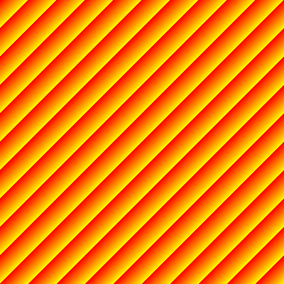
Example: Green Polar
More compactly:
import spire.math.sqrt

val m = 200

val greens = (0 until m).map( i =>
  Color(0, ((i / m.toDouble) * 255).toInt, 0)
).toArray

val gpPca = PixelatedColoredArea(
    (x0: Double, x1: Double, y0: Double, y1: Double) => sqrt(x0*x0 + y0*y0),
    (v: Double) => greens(v.toInt % m),
    400, 400,
    0d, 1000d,
    0d, 1000d)
Create the PNG
import axle.awt._
import cats.effect._

gpPca.png[IO]("docwork/images/green_polar.png").unsafeRunSync()
Future Work
- WebGL
- SVG Animation
- Box Plot
- Candlestick Chart
- Honor graph vis params in awt graph visualizations
axle.web.TableandHtmlFrom[Table[T]]- Log scale
SVG[Matrix]BarChartVariable width bars- Horizontal barchart
KMeansVisualization/ScatterPlotsimilarity (at least DataPoints)SVG[H]for BarChart hover (wrap with \<g> to do getBBox)- Background box for
ScatterPlothover text? - Fix multi-color cube rendering
- Bloom filter surface
- Factor similarity between SVG and Draw?
- Re-enable
axle-jogl
- May require jogamop 2.4, which is not yet released
- Or possibly use jogamp archive
-
See processing's approach in this commit
-
Unchecked constraint in PlotDataView